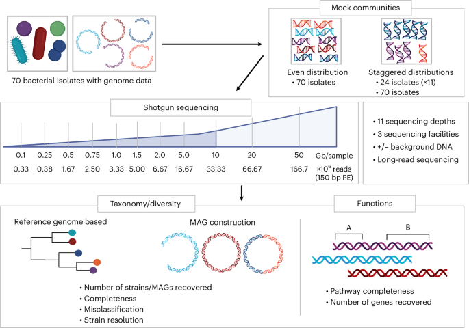
Shallow metagenomics enables reliable reference-based taxonomic profiling
We first investigated the impact of sequencing depth on taxonomic composition. For the three main mock communities (Mock-even-70, Mock-stag-24 and Mock-stag-70), reads were detected for all reference genomes already at 0.1 Gb. To obtain an overview of genome coverage, completeness categories were compared between the sequencing depths. At 0.1 Gb, most of the genomes (63–91%) had a low coverage (0–25 %) (Fig. 2a). Genome coverage increased substantially until 5 Gb of sequencing, with a clear effect of mock community complexity. Most genomes reached >90% coverage at 5 Gb in Mock-even-70 and Mock-stag-24. However, in Mock-stag-70, coverage continued to increase gradually from 5 Gb (36% of genomes at >90% coverage) to 50 Gb (64%), although 11 genomes—added at 0.001 ng (0.00046‰) to 0.1 ng (0.0046%)—still had low coverage (0–25%) at the latter sequencing depth.
a, Number of reference genomes per category of coverage by metagenomic reads (colour gradients) for Mock-even-70, Mock-stag-24 and Mock-stag-70 (top to bottom) at up to 11 sequencing depths (x axis). b, Coefficients of variation of relative abundances of the 70 strains in 10 in silico datasets for each sequencing depth, subsampled from Mock-stag-70 sequenced at 50 Gb. The coefficients of variation between the sequencing depths were tested statistically using a Kruskal–Wallis rank-sum test with Benjamini–Hochberg correction (see P values in Supplementary Data 5). The lower and upper border of the boxes represent the 25th and 75th percentile, and the centre line indicates the median. Whiskers represent the highest and lowest values excluding outliers. Large black points represent outliers. Small grey points show the coefficients of variation between the ten mock communities for the 70 strains at each sequencing depth. c, Difference (delta values) between measured relative abundances and theoretical values (x axis) for the three mock communities after taxonomic assignment using either the reference genomes (blue) or MetaPhlAn4 (red). In the MetaPhlAn analysis, only the taxa that matched reference genomes at the species level were considered.
Source data
Looking at individual strains (Extended Data Fig. 3), the lowest coverage in Mock-even-70 at 0.1 Gb was 3.34% for Phocaeicola sartorii CLA-AV-12 and the highest 58.7% for Bacteroides uniformis CLA-AV-11, which reached 99% coverage already at 0.75 Gb. Full genome coverage (100%) was achieved only at 10 Gb for Veillonella intestinalis CLA-AV-13. In Mock-stag-24 and Mock-stag-70, higher coverage was associated with increasing DNA concentration. The reference genomes with the lowest concentration in Mock-stag-24 (0.01%, 0.04 ng) had a minimum coverage of 0.53% at 0.1 Gb and a maximum coverage of 34.21% at 10 Gb. In Mock-stag-70, the low-abundance genomes—0.1 ng (0.0046%) to 0.001 ng (0.00046‰)—reached 0.8–21.8% coverage at the highest sequencing depth (50 Gb), whereas the genomes of the five strains with the highest DNA amounts (>4.6%) achieved 40.50–98.25% coverage already at 0.1 Gb.
Next, we assessed the relative abundance of strains and compared them with their theoretical values. The overall relative abundance profiles of Mock-even-70, Mock-stag-24 and Mock-stag-70 showed no significant impact of sequencing depth (P = 0.78, 1.0 and 1.0, respectively; Kruskall–Wallis test) (Supplementary Figs. 1 and 2). In addition, bioinformatic subsampling of Mock-stag-70 sequenced at 50 Gb (ten replicates) showed that variations in the relative abundance of individual species were low (average coefficients of variation <5%), with increasing variability at lower sequencing depths (Fig. 2b; see statistics in Supplementary Data 5).
As reference genomes are not available for metagenomic analysis in most studies, the mock communities were also taxonomically analysed using the commonly used profiler MetaPhlAn10, hereon referred to as the non-supervised approach. Overall, the taxonomic assignment in this approach was less sensitive, that is, fewer species were detected. In Mock-stag-24, one strain with low concentration (0.1%, 0.4 ng, Hominilimicola fabiformis CLA-AA-H232) was not detected (Supplementary Fig. 4). In Mock-even-70, 59 species were assigned using MetaPhlAn4, including 47 that matched a reference genome at the species level. In Mock-stag-70, 53 taxa were detected, 44 of which had a species-level match (Supplementary Figs. 3 and 5). The non-supervised approach also showed higher variance from the targeted relative abundances, particularly at lower sequencing depths and with increasing complexity of the mock communities (Fig. 2c; see statistics in Supplementary Data 5).
In summary, reference-based detection of strains is possible with as little as 0.5 Gb of sequencing, but achieving high coverage of reference genomes requires more data (>5 Gb) under the conditions tested. Relative abundance profiles were not substantially affected by sequencing depths for most of the strains. By contrast, non-supervised taxonomic assignment was less sensitive, with fewer species detected.
De novo strain level analysis requires deep sequencing and generates chimeras
Strain-level resolution was evaluated using four Escherichia coli and Phocaeicola vulgatus strains in Mock-even-70 (Extended Data Fig. 1). All strains were detected at 0.1 Gb and achieved >75% genome coverage at 5 Gb and >98% at 10 Gb (Extended Data Fig. 4a). P. vulgatus strains showed similar coverage increase, reflecting their high average nucleotide identity (ANI) values (Extended Data Fig. 4b). For E. coli, the two strains with highest ANI (99.97%) displayed overlapping coverage curves, whereas the more divergent strain CLA-AD-1 (ANI <97%) exceeded 99% coverage already at 2 Gb. By contrast, MetaPhlAn4 detected only one strain per species across all sequencing depths in both Mock-even-70 and Mock-stag-70 (Supplementary Figs. 3 and 5).
Because reference datasets are often unavailable, genomes were reconstructed de novo by assembling metagenome-assembled genomes (MAGs) in each sample. The number of MAGs increased with sequencing depth across all mock communities (Fig. 3a and Extended Data Fig. 5). At high depths, more MAGs than reference genomes (dashed line) were recovered, yet some references remained unrepresented. The number of MAGs per reference genome also rose with sequencing depth, with ≥2 MAGs observed for 22, 12 and 29 references in Mock-even-70, Mock-stag-24 and Mock-stag-70, respectively (Extended Data Fig. 6), indicating splitting into multiple MAGs rather than coalescence into single high-quality genomes.

a, Strain analysis based on the MAGs assembled in Mock-even-70 (top) and Mock-stag-24 (bottom) at each sequencing depth individually. The number of bins assembled from the shotgun data is shown (left, dark blue), as well as the number of reference genomes matching MAGs (coverM) (right, lighter blue), indicating that multiple MAGs were reconstructed for some mock species. The reference genome with the highest coverage by MAG reads was chosen as representative of that MAG. b, Number of high-, medium- and low-quality MAGs assigned to either one (blue) or several (red) reference genomes (with coverM using a cut-off of >0.25% coverage of reference genomes). c, Three exemplary high-quality (>90 % completeness, <5% contamination) (hq) MAGs (dark grey, outer circle) reconstructed from Mock-even-70 at 10 Gb. They were aligned to the reference genomes they covered by more than 0.25% to illustrate different categories of chimerism. The predominantly covered reference genome is depicted in blue, while chimeric sequences of further reference genomes (inner circles) are shown in red. d, Number of hqMAGs assigned to one reference genome (blue) or more reference genomes (orange) for the ten different Mock-stag-24 (v1-10) with varying reference genome abundance distribution. MAGs were constructed with either a single-coverage (bright colours) or a multicoverage (darker colours) binning approach. Statistics: Kruskal–Wallis rank-sum test; ***P = 0.0003871. NS, not significant. e, Number of hqMAGs constructed from contigs assembled with either MEGAHIT or metaSPAdes for Mock-stag-70. The MAGs were then assigned to one (green) or more (red) reference genomes as above. f, High-quality MAGs binned from assemblies generated with either MEGAHIT or metaSPAdes using ten datasets at 10 Gb subsampled in silico from 50 Gb. Bars are mean values; whiskers are standard deviations. Statistics: Wilcoxon rank-sum test (two-sided); *P = 0.012. g, Number of hqMAGs binned from assemblies acquired by long-read sequencing of Mock-stag-70 and categorized as in e.
Source data
To clarify the unexpected number of MAGs and their multiplicity per genome, we assessed their origin by grouping them by quality and assigning contigs to reference genomes (>0.25% coverage threshold). In Mock-even-70 at 10 Gb, 10 of 23 high-quality MAGs (hqMAGs; completeness >90%, contamination <5%) were assigned to multiple genomes (Fig. 3b), with multigenome assignments increasing as MAG quality decreased. GTDB taxonomy agreed with assignments to the reference genomes (Supplementary Data 4). Despite four E. coli strains in Mock-even-70, only one MAG (assigned to E. coli CLA-AD-1) was recovered per dataset >1 Gb (except at 2 Gb, where an additional low-quality MAG appeared). Similarly, although four P. vulgatus strains were present, only one MAG was reconstructed at 5 and 10 Gb, primarily assigned to P. vulgatus strain HDF; therefore, strain delineation was not achieved (Supplementary Data 4).
In Mock-stag-24, a single hqMAG was assembled at 0.75 and 1 Gb (Fig. 3b), primarily assigned to the genome with the highest concentration (40 ng, Thomasclavelia ramosa CLA-JM-H52; ≥95% coverage). With increasing sequencing depth, hqMAGs from lower abundant genomes emerged (Supplementary Data 4). Unexpectedly, single-origin MAGs were more frequent at lower quality, whereas at 10 Gb, half of the hqMAGs were chimeric.
To illustrate chimerism, three hqMAGs (Mock-even-70, 10 Gb) were aligned to the reference genomes they covered >0.25% using blastn (Fig. 3c). MAG 54 matched a single genome (>98% coverage), MAG 16 included fragments of a second genome, and MAG 40 was highly chimeric, comprising sequences from 12 genomes (10 of which are shown, ranked by decreasing coverage from the outer to the inner circle). At 10 Gb, the mean/maximum number of reference genomes per hqMAG was 2.3/12 (Mock-even-70), 1.5/2 (Mock-stag-24) and 2.1/5 (Mock-stag-70) (Supplementary Data 4).
As multicoverage binning was shown to increase the number and quality of MAGs11, we sequenced (10 Gb) ten additional Mock-stag-24 communities (v1-10) with varying reference genome distribution (Supplementary Data 1). Compared with single-coverage binning, significantly more hqMAGs per mock community were assigned to only one reference genome using multicoverage binning (Fig. 3d, blue dots), but chimeric MAGs still occurred in half of the communities (Fig. 3d, orange dots).
To further assess ways to enhance MAG reconstruction, the most complex community (Mock-stag-70) was used to compare assemblers (MEGAHIT versus metaSPAdes) and sequencing technologies (Illumina short reads versus Nanopore long reads). MetaSPAdes assemblies produced more single-origin hqMAGs, especially ≥10 Gb (+1 at 10 Gb, +10 at 20 Gb, +5 at 50 Gb), a result confirmed by in silico subsampling analyses (Fig. 3e,f). Long-read sequencing yielded the highest proportion of single-reference hqMAGs (14 of 15 at 10 Gb; 18 of 22 at 50 Gb) (Fig. 3g).
To test whether chimeric sequences are generated already during the assembly process, contigs were assembled from the 10, 20 and 50 Gb data using either MEGAHIT or metaSPAdes and were aligned to the reference genomes using blastn (Extended Data Fig. 7). Most contigs mapped to a single reference species (average of three sequencing depths: MEGAHIT, 91.1 ± 1.6%; metaSPAdes, 93.5 ± 1.0%), suggesting that 6.5–8.9% misassembled contigs contributed to the reconstruction of chimeric MAGs.
In summary, when high-quality references are available, read mapping enables strain-level analysis of shallow metagenomes. By contrast, de novo MAG reconstruction produces chimeric genomes—even at supposed high quality—due to both assembly and binning. Chimerism was partially reduced by multicoverage binning, strain-aware assembly (metaSPAdes) and long-read sequencing. These findings suggest that strain diversity in MAG catalogues is artificially inflated.
Functional coverage is limited by shallow sequencing
Because functional profiling motivates metagenomics over 16S rRNA gene amplicon sequencing, we evaluated sequencing depth requirements for pathway and gene-based analyses.
Kyoto Encyclopedia of Genes and Genomes (KEGG) pathway completeness (percentage of detected KEGG Orthologs per pathway) was assessed for pathways present in the reference genomes (Extended Data Fig. 8). Among 178 pathways included in the analysis by KEGG-Decoder12, 121 (Mock-even-70, Mock-stag-70) and 118 (Mock-stag-24) were represented in the references. At 10 Gb, a maximum of 80 (Mock-even-70), 77 (Mock-stag-24) and 81 (Mock-stag-70) pathways were complete with the two assembly methods tested (Extended Data Fig. 8). One pathway was not detected in staggered mocks, and 39–41 pathways remained incomplete. Average pathway completeness increased with sequencing depth (Fig. 4a), exceeding 80% at 2 Gb (Mock-stag-70) and 5 Gb (others), then plateauing (+3.7–7.8% at maximum depth).

a, Average KEGG pathway completeness of Mock-even-70, Mock-stag-24 and Mock-stag-70 using contigs assembled with MEGAHIT, and Mock-stag-70 using contigs assembled with metaSPAdes. b, Top: fraction of predicted proteins from the reference genomes covered by the metagenomic assemblies (MEGAHIT) for three different mock communities at the respective sequencing depths. Bottom: reads of Mock-stag-70 were additionally assembled using metaSPAdes. c, Average coverage of functions of the reference genomes by ten in silico datasets, subsampled to ten different sequencing depths each from Mock-stag-70 sequenced at 50 Gb. Bars are mean values; whiskers are standard deviations. Statistics: Kruskal–Wallis rank-sum test with Benjamini–Hochberg correction (see P values in Supplementary Data 5).
Source data
To account for functionally unassigned proteins, detected protein sequences were compared with the repertoire of the reference genomes (Mock-70: 227,543; Mock-stag-24: 82,992 protein sequences). Protein sequence recovery rose to 94.7% in Mock-even-70 (+22.9% from 5 to 10 Gb) but plateaued at 5 Gb in Mock-stag-24 (+12.9%) (Fig. 4b). In Mock-stag-70, coverage reached 55.5/58.3% at 10 Gb and increased only to 71.8/73.8% at 50 Gb (MEGAHIT/metaSPAdes). In silico subsampling of Mock-stag-70 (0.1–20 Gb) confirmed depth-dependent functional recovery with low replicate variation (Fig. 4c; Wilcoxon rank-sum test: Supplementary Data 5).
In summary, ~5 Gb sufficed for functional pathway-level analyses across mock communities, whereas comprehensive protein-level recovery required greater sequencing depth depending on community complexity.
Impact of sample processing and background DNA
To assess wet-lab effects on shallow metagenomics results, DNA libraries were prepared in two facilities using different protocols. In addition, Mock-even-70 and Mock-stag-24 were spiked with DNA isolated from gut content of germ-free mice to simulate host DNA, or left unspiked.
Relative abundance profiles showed distinct clustering owing to both factors (background DNA, facility), with more pronounced effects linked to differences in library preparation protocols between facilities (Fig. 5a). Within a condition (background DNA/facility pair), the extreme sequencing depths (0.1 and 10 Gb) tended to be most distant from each other. The relative abundance profiles of Mock-stag-24 prepared in facility 1, which used more template DNA (100 ng versus 1 ng) and a lower number of polymerase chain reaction (PCR) cycles (5 versus 12), were less sensitive to the effects of sequencing depth when background DNA was present (Fig. 5a, bottom).

a, Principal component analysis (PCA) plot of relative abundance profiles in Mock-even-70 (top) and Mock-stag-24 (bottom). PERMDIST, analysis of multivariate homogeneity of group dispersions; PERMANOVA, permutational multivariate analysis of variance. b, Difference in coverage of reference genomes between facility 1 and facility 2 (left) and samples with or without bgDNA (right) for Mock-even-70. c, As in b for Mock-stag-24. The reference genomes were ranked (from top to bottom) according to increasing DNA amount in the mixture, as indicated by the colour gradient (from blue to red; 0.04, 0.4, 1, 2, 4, 10, 20 and 40 ng).
Source data
Wet-lab effects on reference genome coverage were assessed using delta values between facilities and background DNA conditions. For Mock-even-70, profiles were consistent at 5–10 Gb regardless of facility or background DNA (Fig. 5b), whereas at ≤2 Gb, coverage varied by up to 39% between facilities and 13% with background DNA. For Mock-stag-24, interfacility variation was additionally influenced by input DNA quantity (Fig. 5c). With a reference genome input >1 ng and >1 Gb depth, variance between facilities dropped below 3.69%. Background DNA showed a similar effect on reference genome coverage, but with a more pronounced influence of the amount of reference genome input DNA: variance was negligible (1.33%) with ≥10 ng DNA and ≥1.5 Gb sequencing depth. For >1 ng DNA per strain, ≥5 Gb was required (total variance 3.23%).
Strain-level relative abundances in Mock-even-70 were mostly consistent between library preparation strategies (Supplementary Fig. 1a), indicating that differences shown in Fig. 5a stem from changes in the relative abundance of a few strains. In Mock-stag-24, deviations from theoretical abundances differed between facilities (Supplementary Fig. 1b): Enterocloster clostridioformis matched expectations in facility 1 but was most abundant in facility 2, whereas T. ramosa dominated in facility 1. This suggests that library preparation, particularly template DNA input and PCR cycles, affected relative abundance profiles.
We further assessed wet-lab effects on predicted protein profiles. Facility 1 yielded more complete functional profiles for both mock communities (Extended Data Fig. 9). Background DNA reduced coverage, although this effect decreased at high sequencing depths in facility 1. Overall, background DNA had a stronger impact with the facility 2 protocol.
In summary, using higher template DNA input and fewer PCR cycles improved the robustness of taxonomic and functional profiles. Increased sequencing depth can partially compensate low DNA input or the presence of non-target DNA.


